Matlab and 1B dynamics for CUED students

In the dynamics course, students are introduced to spring and damper systems. The formulae describing these are in CUED's "Mechanics Databook". Here matlab is used to illustrate the behaviour that's summarised on pages 6-9 of the databook.

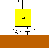
A single mass

For a system where

• m = mass
• f = force
• k = stiffness
• λ = damping

the mechanics databook (p.8) gives the formula

y''/ω² + 2ζy'/ω_n + y = x

where ζ (the damping ratio) is λ/2*sqrt(km), and ω_n (the natural frequency without damping) is sqrt(k/m). Matlab can solve this ODE. If you put the following code into a file called springs.m and run it, you'll get a graph rather like the one on p.7 the data book. Note that I've changed the notation - removing the greek characters and adding digits to the variables so that we can deal with more masses in the future.

function springs
m1=10;
c1=10; % damping
k1=10; % stiffness
f=10; % initial force
x=f/k1;
dampingratio=c1/(2*sqrt(k1*m1));

% Without damping, the natural frequency is w
w=sqrt(k1/m1);

% Y=x/(2*dampingratio*sqrt(1-dampingratio*dampingratio))
natfreq=sqrt(k1/m1)
wdamped=natfreq * sqrt(1-dampingratio*dampingratio)

initial = [0; 0];

for para=[0, 0.1, 0.25, 0.5, 1, 1.5]
     [T,Y] = ode23(@yprime2, [0, 20], initial,[],x,w,para);
     plot(T,Y(:,1)/x);
     hold on
end

function dy = yprime2(t,y,x,w,dampingratio)
   dy= [y(2);  - 2*dampingratio*y(2)*w - y(1)*w*w + x*w*w];

See the Matlab and ODEs page for details about the maths.

On p.6 of the databook 2 more formulae are introduced

• Critical damping is the damping strength that is just enough to prevent any oscillation. λ_crit = 2mω_n
• The natural frequency when there's damping (ω_d) is ω_n/sqrt(1- ζ²)

Of interest is the maximum displacement (see p.8 of the databook). If ζ < 1/sqrt(2) this will be X/(2ζsqrt(1-ζ²)) when ω/ω_n = sqrt(1-2ζ²) (the resonant frequency)

The formulae on p.8 are implemented in the matlab routine below. If you put the following code into a file called springs2.m and run it, you'll get a graph rather like the first one on p.9 of the data book. The lines on the graph correspond to ζ (the damping ratio) having the values 0.1, 0.2, 0.3, 0.5, 1, and 1.5.

function springs2
m1=10;
k1=10; % stiffness
natfreq=sqrt(k1/m1);
clf

freqrange=0.01:0.1:2;

for dampingratio=[0.1 0.2 0.3 0.5 1 1.5]
        if dampingratio < 1/sqrt(2) ;
           wmax= natfreq*sqrt(1-2*dampingratio^2);
           responsemax=1/(2*dampingratio*sqrt(1-dampingratio^2));
           disp(sprintf('max response for dampingratio=%.3f',dampingratio))
           disp(sprintf(' is %.3f at freq=%.3f', responsemax, wmax))
           plot(wmax,responsemax,'or');
        end
     element=1;
     for freq=freqrange
               y(element)=realform(natfreq, dampingratio, freq);
               element=element+1;
     end
      plot(freqrange,y)
      hold on
end


function y=realform(omegan, dampingratio, omega) 
 omegaratio=omega/omegan;
 y= 1/sqrt((1-omegaratio^2)^2 + (2*dampingratio*omegaratio)^2);

The following code uses the "real form" formula on p.8. When put into a file called springs3.m it should generate something similar to the lower graph on p.9 of the databook. The lines on the graph correspond to ζ (the damping ratio) having the values 0.1, 0.2, 0.3, 0.5, 1, and 1.5.

function springs3
m1=10;

k1=10; % stiffness
natfreq=sqrt(k1/m1);
clf

freqrange=0.01:0.1:2;

for dampingratio=[0.1 0.2 0.3 0.5 1 1.5]   
element=1;
for freq=freqrange
          y2(element)=tanphi(natfreq, dampingratio, freq);
          element=element+1;
end
 y3=atan(y2)*180/pi;
 
 y3(y3>0) = y3(y3>0)-180;
 plot(freqrange/natfreq,y3)
 hold on
end
 
function y=tanphi(omegan, dampingratio, omega) 
     omegaratio=omega/omegan;
     y= (-2*dampingratio*omegaratio)/(1-omegaratio^2);

n.b. The maths on this page should display ok on-screen. It may well not print out properly