Matlab by Example

This document attempts to introduce you to matlab by leading you through a useful task, stopping off for some sightseeing on the way. If instead you want a tutorial, then Mathworks' own is as good as any. Some other references are at the end of this document.

Suppose you have a text file of data - 3 numbers per line - from an experiment where values have been obtained at various 2D position. A typical text line is

    45 77 12.78

which means that at (45, 77) the value's 12.78. This example will show you how to

• Read the values into Matlab
• Eliminate outliers and duplicates
• Show the z values as a 2D surface
• Find a best-fit mathematical function for the data
• Save the resulting data
• Make a movie

Read the values into Matlab

First download the data file into a file called data.txt. Start matlab and use cd to change directory (i.e. change what folder you're in) so that you're where the data file is. For example, if the file is in a folder called Downloads, type cd Download in Matlab

Type

  load data.txt

Typing

  whos

will show you that there's now a variable called data

Type

  data

and you'll see the values. data is a matrix. In fact, just about everything in matlab is a matrix, so once you can create and manipulate them you're well on the way to mastering matlab.

Matrix creation

Here are some ways of creating matrices. Note that you don't have to explicitly create matrices before using them, and you needn't specify their sizes - they can grow on demand.

• x=[2 6 7] - create a row vector
• x=[x 8] - add another element to x
• x=[2 ; 6 ; 7 ] - create a column vector
• x=1:6 - create a vector with elements 1, 2, 3 ...6
• x=1:0.5:6 - create a vector with elements 1, 1.5, 2, 2.5 ... 6
• x=linspace(1,6,11) - create a row vector with 11 equally spaced elements running from 1 to 6
• x=ones(4,5) - create a matrix full of 1s with 4 rows and 5 columns
• x=1:3; y=4:6; z=[x y] - join 2 vectors
• x=1:3; bigx=repmat(x, 2, 3) - replicate x twice vertically and 3 times horizontally

Matrix manipulation

Before we continue, let's try some matrix operations.

• size(data) - gets the number of rows and columns. Note that it returns a matrix called ans. We could instead do

     s=size(data)
  

  to put the answer into s. Now s(1) (the 1st element in the array) will be 106 and s(2) will be 3. To suppress screen output, put a semi-colon on the end of the line.
• data(:,1) - shows the 1st column. data(1,:) shows the 1st row. data(:) returns all the elements as a single column.
• data2=data+5 - returns a new array whose elements are each 5 more than data's elements.
• data+data2 - adds the matrices
• data' - returns the transpose of data. Typing size(data') shows you the size of the transpose
• data' * data - multiplies a 3x106 matrix by a 106x3 matrix to give a 3x3 matrix.
• data.*data2 - (note the dot) multiplies each element in data by the corresponding element in data2. The matrices need to be the same size.

Matrix functions

Matlab has many functions. To find out more about a particular function, type help followed by the function name.

• sum(data) - sums each column.
• mean(data) - finds the mean of each column. mean(data(:)) would find the mean of the whole matrix (though that's not useful to us in this situation).
• max(data) - finds the maximum number in each column

Eliminate outliers and duplicates

Any experimental data is likely to contain erroneous or duplicate data. Here we'd first like to eliminate duplicate rows. Whenever you want to find out how to do something and you can think up a keyword you can use lookfor. So

  lookfor duplicate

will look for routines whose descriptions mention "duplicate". Alas there are none. So let's try this

  lookfor unique

This displays several routines. Typing

  help unique

tells us the details. So type

  udata=unique(data,'rows');
 

to create a new matrix with unique rows. It also sorts the rows. Sometimes we don't want that, but it's ok here.

Let's suppose that all z data less than -5 is bogus. We'll set these values to 0. One way to do this would be to use a for loop checking each value much as in a language like Fortran. Here's the code to do that

but there's a quicker way, using the find command.

  toosmall=find(udata < -5)

will return the locations of all the elements in udata(:) that are less than 5. Doing

  udata(toosmall)=0

will set all those elements to 5. We could do this all in one line

  udata(find(udata < -5))=0

udata should now have 101 rows.

Creating commands

Until now you've been typing commands on the matlab command line. If you put these commands into a file into a file (called mycommand.m, say - the suffix is important), then typing mycommand will run the commands in the file. Any text in the file to the right of a % character is ignored. From now on you might prefer to create a file, add new commands to it and run the file. Use clear to clear out variables before re-running. Use close to close all graphics windows. Everything so far could be done using the following file

Much of Matlab is compiled code, though there are many *.m files too. If you type

  which load

(asking where the load command is) you'll see that load is built-in (it's compiled code) but

  which flipud

shows the location of flipud.m which you can look at by typing type flipud. It's only 4 lines of code - see if you can understand it.

Show the z values as a 2D surface

Let's first create some vectors to aid code legibility

Matlab has several ways to plot 3D data. First try

   plot3(xvalues, yvalues, zvalues ,'.')

Note that plot3 (like nearly all matlab commands) can cope with vector arguments. The final '.' puts a dot at each data point.

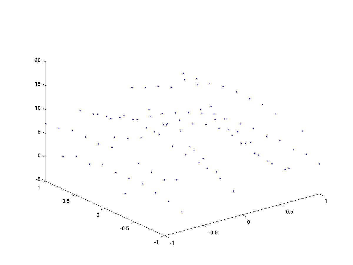
The results aren't easy to visualize. We'd like a surface. For that we need to do more work because some of the more useful matlab commands require the data to be on a regular grid. You can prepare this data for use with the griddata command

% First define a regular grid.
% We'll set up a 20x20 grid
steps = linspace(-1,1, 20);
[XI,YI] = meshgrid(steps, steps);
% XI and YI will both be 20x20. XI contains the x-coords of each point 
% on this new grid, and YI contains the y-coords.

% now interpolate - find z values at each of these grid points
ZI = griddata(xvalues, yvalues, zvalues,XI, YI);

% Display this as a surface
surf(XI,YI,ZI);
hold on ; % this stops the next command clearing the graphics window
% plot the original data too
plot3(xvalues, yvalues, zvalues,'.')

You should get a figure like this

Note that during interpolation, matlab warned that the data contained lines that have different z values for the same (x,y) point. It used the mean z in such situations.

Find a best-fit mathematical function for the data

We might already have in mind a model for the data. For this data, the z values peak at (0.0) and seem to depend on x periodically, so I'm going to try to fit the data to a formula like this

  A1*sin(A2*x) + A3./sqrt(0.5+x.^2 + y.^2);

and I'd like to find constants A1, A2, and A3 such that the values of this expression are as close to z as possible. Matlab has several optimisation routines. I'm going to use lsqnonlin (which you might not have - see later). To use this we have to set the problem up appropriately. We need to specify initial conditions and an expression to minimize. The optimisation functions are rather technical, so I won't go into details - they're online.

a0=[10 10 10 ]; % initial conditions for A1, A2 and A3 - just a guess
% the next line uses 'anonymous functions'. It sets up a function f
% that takes a (containing A1, A2, A3) as input. 
% It's this function that will be minimized
f=@(a) a(1)*sin(a(2)*XI) + a(3)./(0.5+sqrt(XI.^2+YI.^2)) -ZI;

% here we can choose options for the optimisation routine.
options=optimset('Display','iter');
% now we optimise. The returned af vector will contain the A1, A2, and A3 we want
af=lsqnonlin(f,a0,[],[], options)

When I run this I get

Is this a good fit? Let's see

Ztheoretical= af(1) * sin(af(2)*XI) + af(3)./(0.5 + sqrt(XI.^2+YI.^2));
max(Ztheoretical(:)-ZI(:))
mean(Ztheoretical(:)-ZI(:)) 

Let's also see this visually. We'll add the theoretical results as a grid. We'll also add titles, and save the result in a jpeg file.

 close; % clear the graphics
 surf(XI,YI,Ztheoretical);
 title('best fit');
 xlabel('x');
 ylabel('y'); 
 colorbar; % add a color-coded key to z values
 print -djpeg -zbuffer demo1.jpg

The result should be something like this

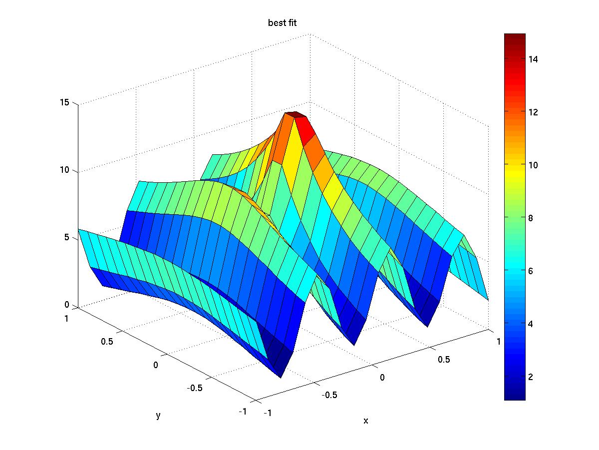
which isn't a perfect fit, but there was noise in the data.

Handle Graphics

We've been changing the figure using commands. We could also have used the menus to change many of these properties. Underlying both of these methods is a third, more direct way. Each part of the figure and the graphs in them has a unique identity number (its "handle") with a set of properties. Type

   get(gca)

and you'll get the list of properties for the current axes. To change any feature you can get its handle then use the set command to change a property. For example, to change the title we can use

   titlehandle=get(gca,'Title');
   set(titlehandle,'FontSize',20);

Toolboxes

Matlab has many add-ons called Toolboxes. lsqnonlin belongs to the Optimisation Toolbox. If you haven't paid for it, you won't have it. Typing

  ver

will show you what's installed, though even if a toolbox is listed, you may not be able to run its routines (the license may have expired, for example).

Fortunately, there are many add-ons that are free. The MATLAB Central: File Exchange has thousands of files to download.

Save the resulting data

Suppose we wanted to store the cleaned, interpolated values in XI, ZI, and ZI. We could do save XI YI ZI 'newdata.txt' but that would save all the elements in the matrices. If we wanted to save in a file with the same form as the original we need to use lower level commands which are like those of the C language.

fp=fopen('newdata.txt','w');
   [rows,cols]=size(XI);
   for i=1:rows
      for j=1:cols
        fprint('%f %f %f \n', XI(i,j), YI(i,j) Ztheoretical(i,j);
      end
   end
fclose(fp);

Make a movie

A figure can be saved into a 'frame' and the frames put together to make a movie. In the code below the viewpoint is changed for each frame. I've forced each frame to be the same size (436 by 344) because otherwise it's hard to make a movie from them.

i=1;
for az=0:-10:-90
 a=viewmtx(az, 30, 60+(az/2));
 view(a);
 M(i)=getframe(gcf,[0 0 436 344]);
 i=i+1;
end
viewmovie(M);

Octave

octave is free, and is similar to Matlab. The code in this example works on linux with octave 3.0.0 until the griddata line. With a different operating system, a newer version of Octave, or extra Octave modules you may have more luck!

References

• CUED's Matlab page
• Mathworks' Getting Started with MATLAB
• the Matlab newsgroup